Applying Experimental Design

by C.J. Keller

Here is a familiar example: a fluid being pumped through a pipe. We are interested in the effect of the system on two responses:

·      Pumping Pressure

·      Pumping energy.

As factors for an designed experiment we select:

·      A hardware option, the pipe size.

·      An operating option, the fluid flow rate.

·      A design option, an additive that is added to the base fluid.

We also suspect that the ambient temperature may have an effect on the responses. We cannot control temperature in our environment but we can measure it. If we were able to control temperature during the experiment, we could assign Temperature as a Subsidiary (Noise, Outer) factor. Because we will not control the temperature we will record it as a Casual Factor.

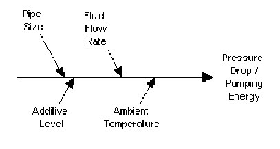
The parameters we want to define are: three main design factors (pipe size, fluid flow rate and additive), a casual factor (temperature), two responses (pumping pressure and energy) and a Run number as a comment column. We could also add other information columns to record operator notes, time, etc..

We suspect that the responses will be influenced by more than linear factor effects, so we want more than two levels for each factor. The factor-levels are the values of each factor to be used in the runs. The design will consist of using combinations of a few levels for each factor, where each combination will be for a run which will produce a response (in this case two responses). If we have only two levels for a factor and we plot a response vs. the two levels, only a straight line can be drawn between them to estimate the effect of other non-tested levels. If there are at least three levels, a curve may be fitted to the three points.

We also suspect that these factors may interact with one-another. If an interaction is present then the response depends not only on adding together the effect from each factor, but also depends on an added effect from the product of two or more factors or on the product of a factor with itself.

There are a number of other factors which may influence the results. We can readily identify some of them: pipe length, pipe interior surface roughness, etc. There may be, and probably are, others which we do not suspect as having an influence. To the extent we can, we will fix or make constant the recognized non-experiment factors. The others we hope will have a random effect, which we will try to enhance by randomizing the order in which the runs are executed.

Consider three pipe diameters: 0.5, 0.75 and 1.00; three flow rates: 1, 3 and 5; and three additive levels: 25, 50 and 75. The choice of at least three levels allows nonlinear effects to be analyzed. Using the same number of levels for all the design factors allows more choices of experimental designs. Using 3 or 5 levels for each factor allows special response surface designs to be available. The program itself can handle any mix of factor-levels.

The casual factor, Temperature, will take on whatever value occurs during each experimental run.

The information for each parameter is defined using a dialog initiated from the parameter information summary screen.

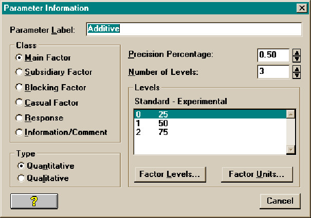
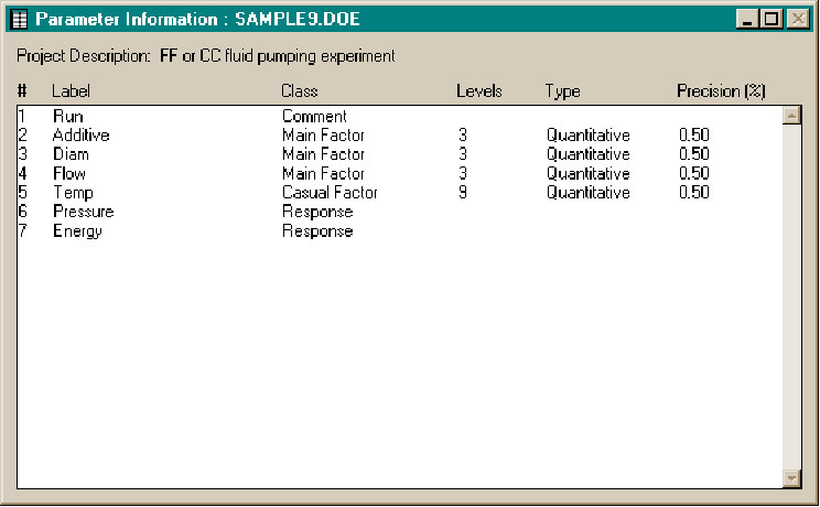
Once the parameters have been defined using the parameter information dialog, the requirements may be defined by specifying an Interaction set. The requirements specify the minimum estimating capability of the proposed design. Interactions not listed may not be capable of being estimated or may be confounded with other factors or interactions.

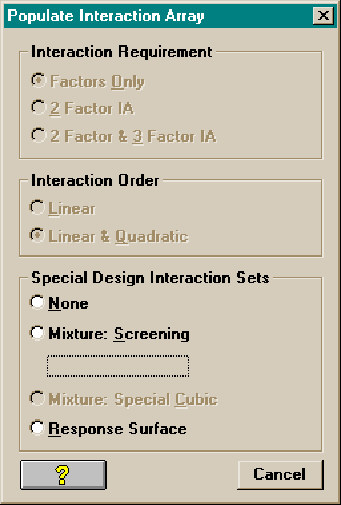
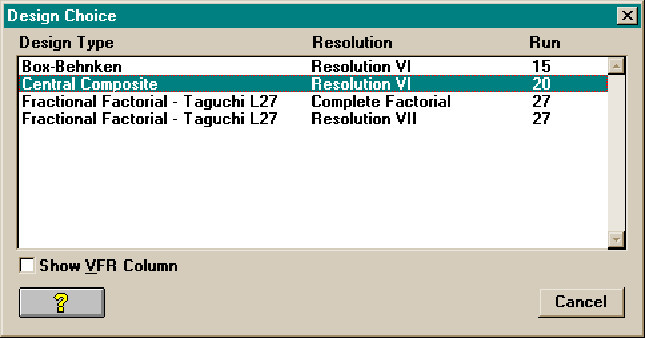
If a limited set of requirements, limited to two-factor quadratic interactions, is selected then a 27-run Complete Factorial design (such as a Taguchi L27) would be available. If a still more modest choice of requirements, a Response Surface set, is chosen a 20-run Central Composite (CC20) design is available.

A default Options in the title bar has selected Experimental Units as our preferred display units. If the User prefers to see designs in a standardized format as is commonly shown in classical references or in the Taguchi notation, those options are also available.

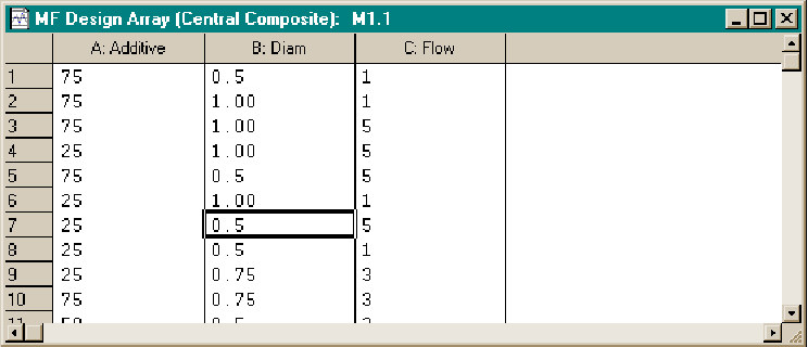
We could if necessary trim some of the 20 center point runs to reduce the design size by selecting: Action + Change Design Array. Both trimming and augmenting of a design can be done by the program so that the User can tailor the number of runs and the performance of the design to his requirements.

So far, our parameters have been defined, a set of requirements selected by specifying an interaction set and a design array chosen.

We can now randomize the run order, produce a Final Design Array for use during the experiment and build a Base Analysis array. The final design array takes the selected and possibly modified design array, combines it with a subsidiary (noise, outer) design if present, provides repeated runs or replicates as selected by options and randomizes the run order. The final design array is then available for printing, copying to the clipboard, exporting to another application and transfer to the Base Analysis array.

The Base Analysis array is where we merge the design with the experimental data. When we get the experimental data, we can enter into the Base Analysis array the Temperature, Pressure and Energy data either by pasting it in or by keyboard entry in the window.

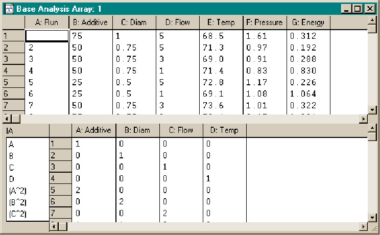
Because we constructed this design using an response surface interaction requirement, we can analyze our data with a response surface analysis as well as with plots and regressions.

An excellent starting plot is for a response vs. the run order. A Pressure vs., Run order plot is shown.

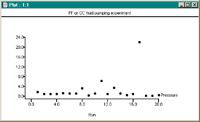
The plot (for this limited data) does not show any obvious order dependency but run 17 may be an outlier or may signal a shift in the fluid flow model. In any event, it should be further evaluated.

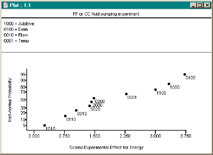
A Half-Normal plot of the effects for Energy shows that the ambient Temperature does indeed have a strong effect on Energy consumption, stronger than Flow. Does this indicate that Flow is not important? No it does not. The HN plot only indicates the change in effect over the range of the data. A thought experiment reducing the flow to zero confirms that the flow is important to the process.

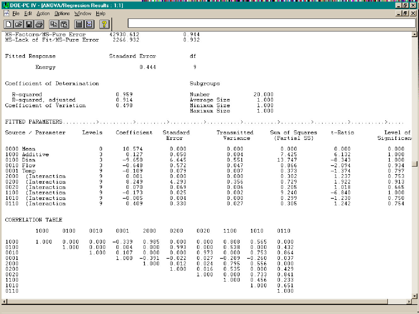
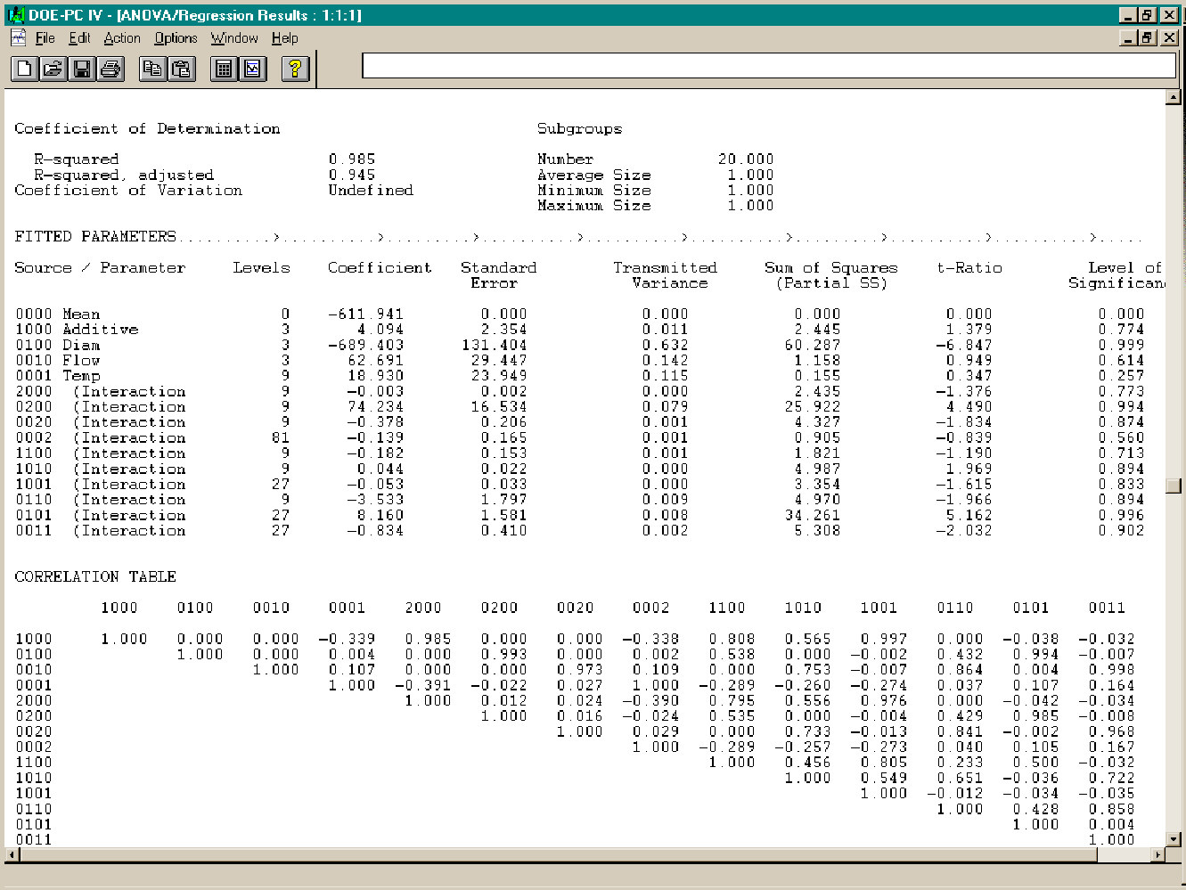
Next a regression analysis is performed using Energy as the response and selecting that the fitted Response be calculated. All the parameters are significant at a probability level of 0.75, except for the quadratic term of Flow. The following image is a partial view of the ANOVA/Regression report window.

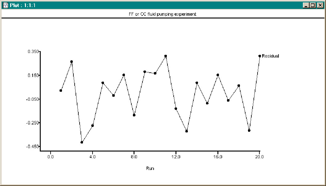
The residual error, the difference between the data response and the fitted response may be calculated by generating a Working Analysis Array from the Base array and then selecting Action + Calculated Response. In that dialog, a calculated response may be generated from one or more of the data columns. If this had been a design suitable for data grouping several Taguchi ratios may also be generated.

A plot of the Energy Residual vs. Run order shows that Run 17, which had previously been identified as a potential outlier, is fitted by the polynomial model about as well as the other points and that further consideration as an outlier is probably not warranted. There is justification for examining the effect of that data run on the model.

Up to this point we have not considered any interactions between the ambient Temperature and the other factors. By selecting Action + Populate Interaction Array + Response Surface, a new interaction list may be generated. It may be tested for feasibility by selecting Action + Audit, which confirms that the data set can support the increased requirements. ( All data sets are automatically checked for adequacy to estimate the requirements list before any numerical operation is attempted.)

A new regression may now be generated based on the expanded interaction list. The expanded model fits the data nicely, but there are some parameters whose level of significance are much less than our previous criterion of 0.75. in particular, the significance of Temperature has been reduced, apparently as a result of including interactions between Temperature and the other factors. The presence of high-significance interactions that include a low-significance linear factor may be an indication of a improper model. That subject is discussed in another note.

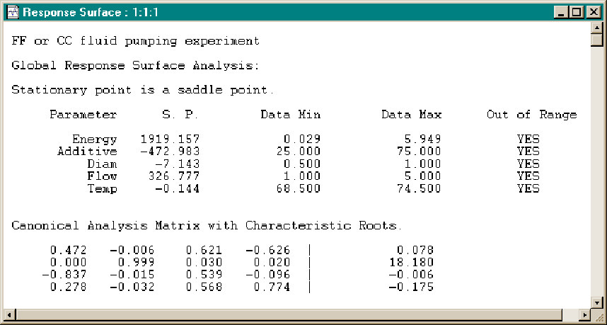
We will keep the current model for the time being and select Action + Response Surface Analysis. The resulting screen shows that there is no Energy maxima or minima within the data range, although there is a saddle point very far from the data.

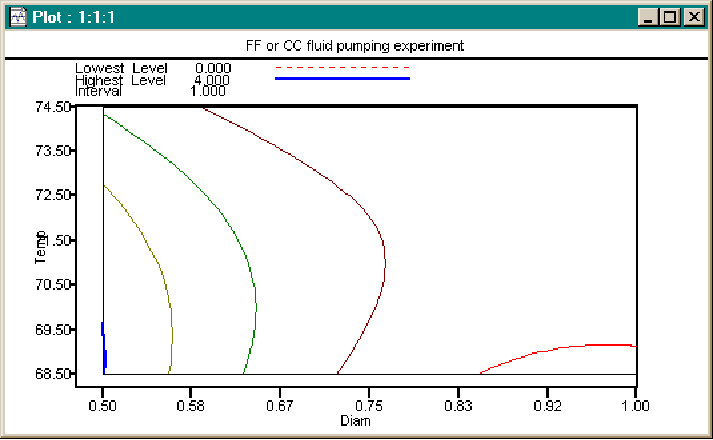
A Contour plot could provide more insight. We have 4 factors, of which only two at a time may be used in a Contour representation of a response; there are 6 such plots, of which only one has fitted values within the data range. The plots themselves may be altered by the selection of the value used for non-plot factors; median data values will be used for the non-plot factors.

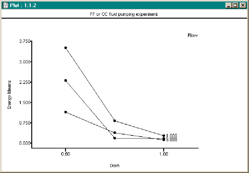
An Interaction chart clearly shows that for the design selection range for Additive and the casual range of Temperature, there is less variation and a lower level of Energy for the largest pipe diameter.

In the real world we would look at more charts, eliminate non-significant factors and interactions from our analysis model and most likely recognize there is not enough data for a robust conclusion, although we certainly do have enough data to make limited conclusions.

One is that the Pressure and Energy responses tend to indicate different selections from among the factor levels for best operation. Another is that larger pipe diameters tend to less variation and lower Energy; low to moderate levels of Additive require less Energy. Some anomalies in the data indicate that we should repeat the experiment for the anomalous data points and replicate a better selected design to get a better measure of variation as well as to look to improving the model.

Learn more about the DOE tools for designed experiments in Six Sigma Demystified (2011, McGraw-Hill) by Paul Keller, in his online Intro. to DOE short course (only $99) or online Advanced Topics in DOE short course (only $139), or his online Black Belt certification training course ($875).