Confidence Intervals

The following is an excerpt from The Quality Engineering Handbook by Thomas Pyzdek, © QA Publishing, LLC.

All statements made in this section are valid only for stable processes, i.e., processes in statistical control. The statistical methods described in this section are enumerative. Although most applications of quality engineering are analytic, there are times when enumerative statistics prove useful. In reading this material, the engineer should keep in mind the fact that analytic methods should also be used to identify the underlying process dynamics and to control and improve the processes involved. The subject of statistical inference is large and it is covered in many different books on introductory statistics. In this book we review that part of the subject matter of particular interest in quality engineering.

III.C.1 Point and interval estimation

So far, we have introduced a number of important statistics including the sample mean, the sample standard deviation, and the sample variance. These sample statistics are called point estimators because they are single values used to represent population parameters. It is also possible to construct an interval about the statistics that has a predetermined probability of including the true population parameter. This interval is called a confidence interval. Interval estimation is an alternative to point estimation that gives us a better idea of the magnitude of the sampling error. Confidence intervals can be either one-sided or two-sided. A one-sided confidence interval places an upper or lower bound on the value of a parameter with a specified level of confidence. A two-sided confidence interval places both upper and lower bounds.

In almost all practical applications of enumerative statistics, including quality control applications, we make inferences about populations based on data from samples. In this chapter, we have talked about sample averages and standard deviations; we have even used these numbers to make statements about future performance, such as long term yields or potential failures. A problem arises that is of considerable practical importance: any estimate that is based on a sample has some amount of sampling error. This is true even though the sample estimates are the "best estimates" in the sense that they are (usually) unbiased estimators of the population parameters.

Estimates of the Mean

For random samples with replacement, the sampling distribution of has a mean µ and a standard deviation equal to . For large samples the sampling distribution of is approximately normal and normal tables can be used to find the probability that a sample mean will be within a given distance of µ. For example, in 95% of the samples we will observe a mean within ±1.96 of µ. In other words, in 95% of the samples the interval

from to will include µ. This interval is called a "95% confidence interval for estimating µ." It is usually shown using inequality symbols:

The factor 1.96 is the Z value obtained from the normal Table 5 in the Appendix. It corresponds to the Z value beyond which 2.5% of the population lie. Since the normal distribution is symmetric, 2.5% of the distribution lies above Z and 2.5% below -Z. The notation commonly used to denote Z values for confidence interval construction or hypothesis testing is Zalpha/2 where 100(1-alpha) is the desired confidence level in per cent. E.g., if we want 95% confidence, alpha=0.05, 100(1-alpha)=95%, and Z0.025=1.96. In hypothesis testing the value of a is known as the significance level.

Example : estimating µ when sigma is known

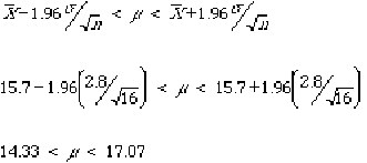
Suppose that sigma is known to be 2.8. Assume that we collect a sample of n=16 and compute X-bar = 15.7 . Using the above equation we find the 95% confidence interval for µ as follows:

There is a 95% level of confidence associated with this interval. The numbers 14.33 and 17.07 are sometimes referred to as the confidence limits.

Note that this is a two-sided confidence interval. There is a 2.5% probability that 17.07 is lower than µ and a 2.5% probability that 14.33 is greater than µ. If we were only interested in, say, the probability that µ were greater than 14.33, then the one-sided confidence interval would be µ > 14.33 and the one-sided confidence level would be 97.5%.

Example: estimating µ when sigma is unknown

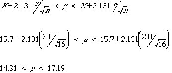
When sigma is not known and we wish to replace sigma with s in calculating confidence intervals for µ, we must replace Zalpha/2 with talpha/2 and obtain the percentiles from tables for Student t distribution instead of the normal tables. Revisiting the example above and assuming that instead of knowing sigma, it was estimated from the sample, that is, based on the sample of n=16, we computed s=2.8 and x-bar = 15.7. Then the 95% confidence interval becomes:

It can be seen that this interval is wider than the one obtained for known sigma. The talpha/2 value found for 15 df is 2.131 (see Table 6 in the Appendix), which is greater than Zalpha/2 = 1.96 above.

Learn more about the Statistical Inference tools for understanding statistics in Six Sigma Demystified (2011, McGraw-Hill) by Paul Keller, in his online Intro. to Statistics short course (only $89) or his online Black Belt certification training course ($875).